MIS 6334 Advanced BA
Project 2: Customer
Analytics using Base SAS

GROUP 11
Chaithanya Sai Srinivas Sabnaveesu – cxs163030
Ritesh Kunisseri Puliyakote – rxk166230
Sindhuja Masiragani – sxm164031
Tejasvi Ramadas Sagar – txs161330
Vinod Premkumar– vmp160030
Table of Contents
Exploring
the dataset
Part I.
Modeling count
data
1. Creation of Count
Dataset
2. NBD
Model
3. Reach, Average Frequency and GRPs
4. Poisson Regression
Model
5. LL Formula - NBD Regression Model
6. NBD Regression Model using
customer characteristics
7. Managerial takeaways between
Poisson Regression and NBD Regression
8. Comparing the models - LR Test
Part II.
Improving the Model
9. Variable Selection
10. Constructing New Variables
11. Interaction Effects
Part
III. Why Certain Customers Prefer Amazon Over BN?
12. Logistic Regression
Part IV.
Summary
13. Insights and Learnings
Appendix
Exploring the dataset:
Data:
The provided data consists of customer purchase
behavior from Amazon and BARNESandNOBLE. The data is provided with customer
demographics along with some other variables like quantity, price, product,
date and domain. As with every other data we have missing values and, so we had
to preprocess even before analyzing the data.
Preprocessing:
While observing the data characteristics, we observed
that the Education has more than 73% missing values, Age has 3 missing values
and region has 46 missing values. So, to handle these variables, we removed
education variable and imputed the age and region variables with its respective
mode values.
Dataset:
Total records:
40,945
We can classify the
variables as below:
Demographic
variables: Education, Region, Household size(hhsz), Age, Income, Child, Race,
Country
ID or Index
variable: UserID
Purchase variables: Quantity(qty), Price, Product,
Domain
Analyzing the variables for and finding missing values:
PROC CONTENTS: The PROC CONTENTS procedure generates
summary information about the contents of a dataset. This procedure is useful
if you want to know basic information about the dataset itself, such as the
variables' names, types, and attributes.
PROC CONTENTS DATA=P2.ABN;
RUN;
Below is the screenshot showing a part of contents obtained
for PROC CONTENTS.

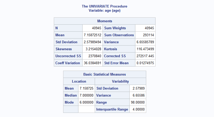
PROC UNIVARIATE: This is a procedure within BASE SAS used
primarily for examining the distribution of data, including an assessment of
normality and discovery of outliers.
PROC
UNIVARIATE DATA
= P2.ABN;
RUN;
PROC FREQ: The PROC FREQ statement is the only required
statement for the FREQ procedure. If you specify the following statements, PROC
FREQ produces a one-way frequency table for all the variables in our data.
PROC
FREQ DATA
= P2.ABN;
RUN;
Education: Age consists of more than 50% missing values which
are represented as 99 in the original dataset.
So, we must decide on this variable whether to include in the rest of
the data or impute these missing values
PROC
FREQ DATA
= P2.ABN;
TABLE
EDUCATION;
RUN;

Age: Age has 3 missing
values which are represented by value 99.
PROC
FREQ DATA
= P2.ABN;
TABLE
age;
RUN;

Region: Region consists of 46 missing values which are
represented by value a ‘*’.
PROC
FREQ DATA
= P2.ABN;
TABLE
region;
RUN;

Modifying original
data:
Based on the above
observations,
LIBNAME proj 'C:\Users\Vinod Prem
Kumar\Documents\My SAS Files\project 2';
data assign1.newfile;
set assign1.data_books;
if education = "99" then education = '.';
if age = "99" then age = ".";
if region = "*" then region = ".";
run;
Part I: Modeling
Count Data
1.
Count number of books purchased from
BN in 2007
proc sql;
create table assign1.count as
select distinct userid, region, hhsz,
age, income, child, race, country, domain,
sum(qty) as total_qty, sum(price) as total_sum
from assign1.newfile
where domain = "barnesandnoble.com"
group by userid, region, hhsz,
age, income, child, race, country;
quit;
Proc Print data=assign1.count (obs=10);
Run;

1.
NBD Model
LIBNAME assign1 'C:\Users\Vinod Prem
Kumar\Downloads';
Proc Print Data=assign1.data_books;
Run;
LIBNAME assign1 'C:\Users\Vinod Prem
Kumar\Documents\My SAS Files\project 2';
Proc Print Data=assign1.newfile;
Run;
Proc sql;
Select count(unique(userid)) from assign1.newfile;
quit; /*Unique User IDs that made purchase from B&N or both*/
Proc sql;
Select count(unique(userid)) from assign1.count;
quit; /*Creating table with
total books and number of people*/
Proc sql;
Create table assign1.nbdModel as Select total_qty, count(userid)
as num_people from assign1.count group by total_qty;
quit; /*Inserting People with 0 number of purchases from B&N*/
Proc sql;
Insert into assign1.nbdModel (total_qty,
num_people) values (0,7639);
quit; /*Sorting the data and printing the first 10 observations for
reference*/
Proc sort data=assign1.nbdModel; by total_qty;
run;
Proc print data=assign1.nbdModel (obs=10);
Run;


1.
Report Reach, Average Frequency and
GRPs
p(X(t)=0)= ( a/a+t ) r =
( 0.1299/0.1299+1 ) 0.09723 = 0.810324813
E(X(t)) = rt/a =
0.09723*1/0.1299 = 0.748498845
Reach = 1-p(X(t)=0) = 1 –
0.8103 = 18.97%
Avg. Frequency =
E(X(t))/Reach*100 = 3.946213827
GRPs = 100*E(X(t)) =
100*0.748498845 = 74.8498845
2.
Poisson Regression Model
LIBNAME assign1 'C:\Users\Vinod Prem
Kumar\Documents\My SAS Files\project 2';
Proc Print Data=assign1.newfile;
Run;
proc sql;
Create Table assign1.table1 as
Select userid, region, hhsz,
age, income, child, race, country, domain, sum(qty) as total_books
from assign1.newfile
group by userid, region, hhsz,
age, income, child, race, country, domain;
quit;
/*---Users that bought
from Barsne&Noble---*/
proc sql;
Create Table assign1.barn as
Select userid from assign1.table1
where domain = "barnesandnoble.com";
quit;
/*---Users that bought
from Amazon---*/
proc sql;
Create Table assign1.amazon as
Select userid from assign1.table1
where domain = "amazon.com";
quit;
/*---Users that bought
from both Amazon and BarnesAndNoble---*/
proc sql;
Create Table assign1.both as
Select * from assign1.amazon intersect
Select * from assign1.barn;
quit;
/*---Users that bought
only from Amazon and not from BarnesAndNoble---*/
proc sql;
Create table assign1.justamazon as
Select * from assign1.amazon
except Select * from assign1.both;
quit;
/*---Adding Demographic
details to AmazonOnly Table---*/
proc sql;
Create Table assign1.justamazondemo as
Select all.userid, all.region,
all.hhsz, all.age, all.income, all.child, all.race, all.country
from assign1.table1 as all, assign1.justamazon as amazon1
where all.userid =
amazon1.userid;
quit;
/*---For the above data,
since no one bought from BarnesAndNoble, total_books=0---*/
data assign1.justamazondemo;
set assign1.justamazondemo;
domain = "amazon.com";
total_books = 0;
run;
/*---Creating Table for
people who bought from BarnesAndNoble along with demographic details---*/
Proc sql;
Create Table assign1.Barndemo as
Select * from assign1.table1
where domain = "barnesandnoble.com";
quit;
/*Combining the
Bndemographic table with amazononlydemographic table to obtain the final table
required for regression*/
Proc sql;
Create Table assign1.final as
Select * from assign1.justamazondemo
union Select* from assign1.Barndemo;
quit;
/*First 10 observations
for the resulting data obtained for reference*/
Proc print data=assign1.final (obs=10);
run;
/*--------------Poisson Regression
for the data abi.final-------------------- --*/
Proc NLMixed Data=assign1.Final;
Parms m0=1 b1=0 b2=0 b3=0 b4=0 b5=0 b6=0 b7=0;
m =
m0*exp(b1*region+b2*hhsz+b3*age+b4*income+b5*child+b6*race+b7*country);
ll=log((m**total_books)*(exp(-m))/fact(total_books));
Model total_books ~ general(ll);
Run;


Maximum LL = 18819
Value of λ0 = 0.9497
Managerial Implications:
As per the above results,
it is observed that region (b1), age (b3), income (b4), child (b5), race (b6)
and country (b7) are significant parameters considering p value at 5%. We can
also observe that the p value for hhsz is more than 0.05.
5. LL Formula - NBD
Regression Model
NBD Regression Model is defined given below:
LL (Log Likelihood) is summation of (Total number of books
purchased * P(Yi=y)) where exp(β’xi) = exp(b1* education + b2*region +b3 *hhsz
+ b4*age + b5*income + b6*child + b7*race + b8*country)
6. NBD Regression Model
using customer characteristics
NBD Regression Model be represented using SAS code as
follows:
Proc NLMixed Data=assign1.Final;
Parms alpha=1 r=1 b1=0 b2=0 b3=0 b4=0 b5=0 b6=0 b7=0;
expB=
exp(b1*region+b2*hhsz+b3*age+b4*income+b5*child+b6*race+b7*country);
ll=
log((GAMMA(r+total_books)/(GAMMA(r)*fact(total_books)))*((alpha/(alpha+expB))
**r)*((expB/(alpha+expB))**total_books));
Model total_books ~ general(ll);
Run;


Maximum LL =
8371.0292
α = 0.1074
r = 0.09814
As per the above
observation, we can say that region (b1), race(b6) are significant. Hhsz (b2),
age
(b3), income (b4), child (b5) and
country (b7) are not significant.
7. Managerial takeaways
between Poisson Regression and NBD Regression
/*---Predicting the values using Poisson Regression
Results---*/
LIBNAME assign1 'C:\Users\Vinod Prem
Kumar\Documents\My SAS Files\project 2';
%let m0 = 0.9497;
%let b1 = -0.1022;
%let b2 = -0.01499;
%let b3 = 0.02511;
%let b4 = 0.01499;
%let b5 = 0.07290;
%let b6 = -0.2083;
%let b7 = -0.1179;
Data PoiFinal (drop = y);
set assign1.Final;
m =
&m0*exp(&b1*region+&b2*hhsz+&b3*age+&b4*income+&b5*child+&b6*race+&b7*country
);
array prob(11) prob0 - prob10;
prob0 = poisson(m,0);
prob10 = 1-prob0;
do y=1 to 9;
prob(y+1)=poisson(m,y)-poisson(m,y-1);
prob10=prob10-prob(y+1);
end;
Run;
Proc means data=PoiFinal mean;
var prob0-prob10;
Run;

Books
|
Actual
|
Predicted
|
0
|
7639
|
4501.02
|
1
|
753
|
3307.826
|
2
|
362
|
1246.635
|
3
|
175
|
320.576
|
4
|
126
|
63.18372
|
5
|
82
|
10.16739
|
6
|
74
|
1.389722
|
7
|
30
|
0.165752
|
8
|
48
|
0.017586
|
9
|
31
|
0.001684
|
10
|
131
|
0.00016
|
Total
|
9451
|


Books
|
Actual
|
Predicted
|
0
|
7639
|
7658.841
|
1
|
753
|
661.8573
|
2
|
362
|
320.4371
|
3
|
175
|
197.7017
|
4
|
126
|
135.1417
|
5
|
82
|
97.79706
|
6
|
74
|
73.39552
|
7
|
30
|
56.49713
|
8
|
48
|
44.30912
|
9
|
31
|
35.25412
|
10
|
131
|
169.7693
|
Total
|
9451
|

/*---Predicting the values using NBD Regression Results---*/
LIBNAME assign1 'C:\Users\Vinod Prem
Kumar\Documents\My SAS Files\project 2';
%let alpha = 0.1078;
%let r = 0.09804;
%let b1 = -0.1035;
%let b2 = -0.00850;
%let b3 = 0.02854;
%let b4 = 0.01730;
%let b5 = 0.05816;
%let b6 = -0.2099;
%let b7 = -0.1015;
Data NBDProb (drop=y);
set assign1.Final;
expB =
exp(&b1*region+&b2*hhsz+&b3*age+&b4*income+&b5*child+&b6*race+&b7*country);
array prob(11) prob0-prob10;
prob0 = (GAMMA(&r+0)/(GAMMA(&r)*fact(0)))*((&alpha/(&alpha+expB))**&r)*((expB/(&alpha
+expB))**0);
prob10 = 1 - prob0;
do y=1 to 9;
prob(y+1)=
(GAMMA(&r+y)/(GAMMA(&r)*fact(y)))*((&alpha/(&alpha+expB))**&r)*((expB/(&alpha
+expB))**y);
prob10=prob10-prob(y+1);
end;
run;
Proc means data=NBDprob mean;
Var prob0-prob10;
run;
Considering the log-likelihood value of Poisson Regression (~
-18819) and NBD Regression (~ -8359) we observe that there is a large
difference between the two results. From this, we can infer that NBD Regression
is a good model as it has better maximum log likelihood value. As is evident
from the graph of the predictions through Poisson Regression and NBD
Regression, NBD regression performs much better in predicting total when
compared to actual values.
Also, we can observe that only region(b1), race(b6) are
significant in NBD regression model whereas region (b1), age (b3), income (b4),
child (b5), race(b6) and country (b7) are significant in the Poisson regression
model.
Possible explanation:-In the Poisson regression model, we
considered only how people differ on a set of available explanatory variables
(We keep the lambda constant), while in NBD regression model, we try to capture
the unobserved variables which might influence the target variables along with
the available explanatory variables. (i.e we varied the 0 across the customers
according to a gamma distribution with parameters r and a)
Only Region was a significant variable in NBD Regression and
it performed better as compared to Race, Age and Income being a significant
variable in Poisson Regression. The explanatory variables are not enough to
capture the actual difference among individuals which we used in Poisson
Regression.
Further explanation: - As we observed, only two variables are
significant in the NBD regression model (region(b1), race(b6)). This change in
output of NBD regression might be a phenomenon of omitted variables’ bias
(unobserved variables). These omitted variables might be correlated with the
included independent variables and the dependent variable. In other words, in
the regression the error term might be correlated with the independent
variables and hence the difference.
To capture the unobserved component of differences among
individuals, we must consider variation of lambda across the population which
we used in NBD Regression. Finally, the LL value decreased to 8358.7726 in NBD
from 18819.0476 in Poisson Regression.
8. Comparing the models
- LR Test
Consider two models A and B, taking thoughts from the
concept that we can arrive at model B by placing k constraints on the parameters
of model A.
Now considering λ0 constant as a constraint for
Poisson regression, let our models be as follows:
Model A: NBD regression
Model B: Poisson regression
Therefore, we use the likelihood ratio test to
determine whether model A, which has more parameters (r and α) fits the data
better than model B.
The null hypothesis is that model A is not different
from model B
Computing test statistic
LR = −2(LLB −
LLA)
=
-2(-18819.0476 -(-8358.7726))
LR = 20920.55
χ2 (.05, k) = χ2 (.05,1)
χ2 =3.84146
Since, LR > χ2 (.05, k), we reject null hypothesis.
Hence, we state that Model A is better than model B.
Therefore, NBD model is better than Poisson regression
model.
PART 2: Improving the
model
9. Variable selection
Explored the variables in SAS Enterprise Miner and found out that
Education had more than 75 percent missing values. So, we did not try to impute
it as it would skew the data. Hence, we rejected the Education variable.
We then ran the PCA on SAS EM without assigning the data
types to the different variables and got the following result:

We ran NBD regression model to find how each variables were
significant
LIBNAME
assign1 'C:\Users\Vinod Prem Kumar\Documents\My SAS
Files\project 2';
data
assign1.newfile;
set
assign1.data_books;
if
age = 99 then
age = 6;
if
country = 1 then
region = 5;
if
region = ' ' and country = 0
then region = 3;
DROP
education count;
run;
proc
genmod data
= assign1.data_books;
model
domain= region hhsz age income child race;
run;

We found that Region, income and race were the most
influential variables for domain.
Variable Country wasn’t adding much value to explain the
variation in the dependent variable. Hence, we tried to analyze if the Country
variable could be eliminated.
Region Variable has 4 bins which represent the US countries. Country
has only US and non-US, we can derive country from Region. So, we added an
extra bin to the Region variable to represent all the non-US countries and
rejected the Country variable.
Now we assigned the data types to all the variables and
rejected the ones which weren’t needed for our analysis. Then ran PCA

We ran NBD
regression model to check for significance values
LIBNAME
proj 'C:\Users\Vinod Prem Kumar\Documents\My SAS Files\project 2';
data
proj.newfile1;
set
proj.data_books;
if
education = "99" then
education = ".";
if
age = "99" then
age = "6";
if
country = 1 then
region = 5;
if
region = ' ' and country = 0
then region = 3;
run;
proc
genmod data
= assign1.newfile1;
model
domain= region hhsz age income child race;
run;

10.
We identified DATE variable our analysis, date can be broken
down into Weekdays and Weekends to give more comprehensive view to our
analysis.
To convert date from calculate day of the week taking wd=1 as
Sunday and wd=7 as Saturday numeric yyyymmdd format to ddMMMyyyy format.
LIBNAME
assign1 'C:\Users\Vinod Prem Kumar\Documents\My SAS
Files\project 2';
From
the question 9, as we know the variable Country is redundant and the data can
be retained by adding a new category to the region which is 5th region for
Non-US (Country = 1) and imputing the region values with the mode value for
missing.
Week day (wd) Variable from Date
variable:
DATA
assign1.ABNWeek;
SET
assign1.newfile;
IF
COUNTRY = 1 THEN
REGION = 5;
IF
COUNTRY = 0 AND REGION = ' '
THEN REGION = 3
;
ORDERDATE
= input(put(date, 8.), yymmdd8.);
format
ORDERDATE date9.;
wd
= WEEKDAY(ORDERDATE);
DROP
COUNTRY DATE;
RUN;
Created
a dataset BNWeekData containing the Quantity classifying Weekend and Weekday
quantity for Barnes and Noble domain.
PROC
SQL;
CREATE
TABLE assign1.BNWeekData AS
SELECT
userid,
CASE
WHEN
Wd=1 THEN
qty
WHEN
Wd=7 THEN
qty
ELSE
0
END
AS
weekendQty,
CASE
WHEN
Wd=2 THEN
qty
WHEN
Wd=3 THEN
qty
WHEN
Wd=4 THEN
qty
WHEN
Wd=5 THEN
qty
WHEN
Wd=6 THEN
qty
ELSE
0
END
as weekdayQty,
ORDERDATE
FROM
assign1.ABNWeek
WHERE
domain="barnesandnoble.com"
;
QUIT;
Dataset
SUMBNWeekData is: Summarizing the data of total quantity purchased on Weekend
and Weekday per User.
PROC
SQL;
CREATE
TABLE assign1.SUMBNWeekData as
SELECT
DISTINCT userid,sum(weekdayQty) as
TotalWeekendQty,
sum(weekendQty)
as TotalWeekdayQty FROM
assign1.BNWeekData GROUP BY
userid;
QUIT;
proc
sql;
create
table assign1.countDate as
select
userid,sum(qty) as total_qty, education, region,
hhsz, age, income, child, race, country, domain,
sum(price)
as total_sum
from
assign1.newfile
where
domain = "barnesandnoble.com"
group
by userid, region, hhsz, age, income, child, race,
country;
quit;
We
have quantity purchases completed on weekdays and weekends. From this data we
can assess what product are purchased on which days of the week. This is also
helpful to run different models again to achieve the finest results to benefit
information that impacts.
PROC
SQL;
CREATE
TABLE assign1.BNWeeKQty AS
SELECT
DISTINCT *,
CASE
WHEN
TotalWeekendQty IS NULL THEN
0
ELSE
TotalWeekendQty
END
AS
TotalWeekendQty,
CASE
WHEN
TotalWeekdayQty IS NULL THEN
0
ELSE
TotalWeekdayQty
END
AS
TotalWeekdayQty
FROM
assign1.countDate as CBN
LEFT
JOIN
assign1.SUMBNWeekData
as SBN
ON
SBN.USERID = CBN.USERID;
QUIT;
Poisson Model
proc
nlmixed data=
assign1.BNWeeKQty;
parms
m0=1 b1=0
b2=0 b3=0
b4=0 b5=0
b6=0 b7=0
b9=0 b10=0
b11=0;
m=m0*exp(b1*education
+ b2*region+b3*hhsz+b4*age+b5*income+b6*child+b7*race+b8*country +
b9*total_sum+b10*TotalWeekendQty+b11*TotalWeekdayQty);
ll =
total_qty*log(m)-m-log(fact(total_qty));
model
total_qty~ general(ll);
run;
Results

Managerial Takeaway
We
can infer from the parameter estimates that the newly constructed variables TotalWeekendQty(b10)
which is Total quantity purchased on weekend and TotalWeekdayQty(b11) which is
Total quantity purchased on weekday are having significant p-value less
than 0.05. This indicates that these variables will impact our analysis.
NBD Regression
PROC
NLMIXED DATA=
assign1.BNWeeKQty;
PARMS
r=1 alpha=1
b1=0 b2=0
b3=0 b4=0
b5=0 b6=0
b7=0 b8=0
b9=0 b10=0
b11=0;
Expn=exp(b1*education
+ b2*region+b3*hhsz+b4*age+b5*income+b6*child+b7*race+ b8*country +
b9*total_sum+b10*TotalWeekendQty+b11*TotalWeekdayQty);
Prob=(gamma(r+total_qty)/(gamma(r)*fact(total_qty)))*((alpha/(alpha+Expn))**r)*((Expn/(alpha+Expn))**total_qty);
ll=Log(Prob);
MODEL
total_qty~ GENERAL(ll);
RUN;

Managerial
Takeaway
With the NBD Regression Model
Maximum LL was improved. We can infer the significant variables in the above
model are Income(b5), total_sum(b9), TotalWeekendQty(b10) which is Total
quantity purchased on weekend and TotalWeekdayQty(b11) which is Total quantity
purchased on weekday are having significant p-value less than 0.05.
Season(season) variable from the
DATE variable
proc
sql;
create
table assign1.countSeasonBN as
select
userid, region, hhsz, age, income, child, race, country, domain, date,
education,
sum(qty)
as total_qty, sum(price) as
total_sum
from
assign1.ABN
where
domain = "barnesandnoble.com"
group
by userid, region, hhsz, age, income, child, race,
country;
quit;
DATA
assign1.SeasonBN;
SET
assign1.countSeasonBN;
length
month $ 2 day $ 2;
date_conv
= put(date,8.);
month
= substr(date_conv,5,2);
day
= substr(date_conv,7,2);
DROP
DATE domain;
RUN;
DATA
assign1.SeasonBN;
SET
assign1.SeasonBN;
IF
month = 01 or month = 02
or month = 03 or month = 04 THEN
season = 1;
ELSE
IF month = 05
or month = 06 or month = 07
THEN season=2;
ELSE
season=3;
RUN;
proc
GENMOD data=
assign1.SeasonBN;
CLASS
season region;
MODEL
total_qty = education region hhsz age income child race country total_sum
season / dist = Poisson link
= log;
run;

Managerial
Takeaway
For the class variables region
and season, with the NBD distribution the significant variables in the above
model are Age, Income, Race, Country, Total_sum, Season. Purchases from the region 1 are more likely
tending towards the BN than from region 2 and 3. In Season 2, people are buying
more from BN than n Season 1 or 2.
Calculating the Loyalty of BN Customers
LIBNAME
P2 'C:\Users\chait\Desktop\Sem3\ABA SAS\Project2\ds';
PROC
sql;
Create
table p2.loyalBN as
SELECT
DISTINCT userid, count(qty) as
CountOfQtyBN
from
p2.newfile
Where
domain= "barnesandnoble.com"
GROUP
BY userid;
QUIT;
PROC
sql;
Create
table p2.loyalTotal as
SELECT
DISTINCT userid, count(qty) as
CountOfTotalQty
from
p2.newfile
GROUP
BY userid;
QUIT;
PROC
sql;
Create
table p2.loyalUsers as
SELECT
Distinct c.userid, c.region, c.hhsz, c.age,
c.income, c.child, c.race, lbn.CountOfQtyBN,lt.CountOfTotalQty
from
p2.lbn as lbn inner
join p2.lt as
lt ON lbn.userid = lt.userid
inner
join p2.ABNWeek as
c ON c.userid = lbn.userid
GROUP
BY lt.userid ;
QUIT;
DATA
p2.loyalty;
SET
p2.loyalUsers;
IF
CountOfQtyBN > (CountOfTotalQty – CountOfQtyBN)
THEN
loyalBN = 1;
ELSE
loyalBN=0;
PercentageOfLoyalty
= (CountOfQtyBN/CountOfTotalQty)*100;
RUN;
proc
genmod data
= p2.loyalty;
class
age income child race region;
model
CountOfQtyBN = age income child race region hhsz /dist
= NBD
link
= log;
run;


Managerial Takeaway
For the class variables age
region race income with the NBD distribution the significant variables in the
above model are Age, Income and Region. Customers
from the region 1 are more loyal compared to region 2, 3 and 4 towards BN. Customers
falling under the band of Age 4 and 10 or Income level 5 are more loyal towards
BN.
11. Interactions
a. Child and Income
proc
genmod data
= assign1.newfile1;
model
domain= region age hhsz income*child race;
run;

As observed from Analysis of Maximum Likelihood Parameter
Estimates table, the interaction of child and income variables does not yield
any significant values as the p value > 0.05.
b. Age and Child
proc
genmod data
= assign1.newfile1;
model
domain= region age*child hhsz income race;
run;
 As observed from Analysis of Maximum Likelihood Parameter
Estimates table, the interaction of age and Child variables does not yield any
significant values as the p value > 0.05.
As observed from Analysis of Maximum Likelihood Parameter
Estimates table, the interaction of age and Child variables does not yield any
significant values as the p value > 0.05.
c. hhsz and Income
proc
genmod data
= assign1.newfile1;
model
domain= region age hhsz*income child race;
run;

As observed from Analysis of Maximum Likelihood Parameter
Estimates table, the interaction of hhsz and Income variables does not yield
any significant values as the p value > 0.05.
PART 3: Certain Customers prefer Amazon over BN. Why?
12. Logistic Regression
LIBNAME
assign1 'F:\6334\aba_project2_data_books';
data
assign1.newfile;
set
assign1.aba_project2_data_books;
if
education = "99" then
education = '.';
if
age = "99" then
age = '.';
if
country = 1 then
region = 5;
if
region = ' ' and country = 0
then region = 3;
run;
proc
sql;
create
table assign1.barntable as
select
distinct userid, region, hhsz, age, income,
child, race, country, domain,
sum(qty)
as total_barn
from
assign1.newfile
where
domain = "barnesandnoble.com"
group
by userid;
proc
sql;
create
table assign1.amzntable as
select
distinct userid, region, hhsz, age, income,
child, race, country, domain,
sum(qty)
as total_amzn
from
assign1.newfile
where
domain = "amazon.com"
group
by userid;
proc
sql;
create
table assign1.final as
select * from
proj.barntable
union
select * from
assign1.amzntable;
data
assign1.final2;
set
assign1.final;
if
domain = "amazon.com"
then do
total_amzn
= total_barn;
total_barn
= 0;
end;
if
domain = "barnesandnoble.com"
then total_amzn = 0;
run;
proc
sql;
create
table assign1.comb as
select distinct
userid, region, hhsz, age, income, child, race, country, sum(total_barn) as
totbarn, sum(total_amzn) as totamzn from
assign1.final2
group
by userid;
run;
data
assign1.finreg;
set
assign1.comb;
if
totbarn > 0 then
flag_barn = 1;
else
flag_barn = 0;
if
totamzn > 0 then
flag_amzn = 1;
else
flag_amzn = 0;
run;
/*
logistic regression for BarnesandNobles*/
proc
logistic data
= assign1.finreg;
model
flag_barn= region hhsz age income child race;
run;
/*
logistic regression for Amazon*/
proc
logistic data
= assign1.finreg;
model
flag_amzn= region hhsz age income child race;
run;
Barnes and Nobles

Amazon

proc
logisitic data = proj.finreg;
class
region age income;
model
flag_amzn = region hhsz age income child race/ selection = forward expb;
run;

Managerial Takeaway:
·
People
from region 4 tends to purchase more from BarnesandNobles than Amazon.
·
People
from U.S. leans towards Amazon over BarnesandNobles
·
Younger
age people prefer Amazon over BarnesandNobles
PART 4:
Summary
13. Insights
and Learnings
· Date: In the dataset the date
variable is in the numeric data type. We converted the date variable to DATE 9.
Format to get insights based on Weekday, Weekend, Seasons and Loyalty
· All the regions are having the Non-Us
(Country = 1) values which is incorrect, we added a new category to the region
as 5 contains Non-Us value.
· We observed that region 2 has not
much sales for BN.
· Learned how to build customized
analytic model using Base SAS
· Understood the difference between
Poisson Regression and NBD Regression Model and how to compare the models using
LR test
· Dataset has 5:1 ratio of amazon is to
BN. Hence, it is biased towards amazon which leads to small contribution for
findings on BN
· Although there are high influential
variables, combining with non-influential variables will not yield any significant
results
· Data preprocessing played a key role
in analyzing the MLE for the given data
· Working on this project and creating
customized BA model using Base SAS has equipped us with the understanding of
analysis of raw data and coming up with actionable recommendations to make
business more efficient